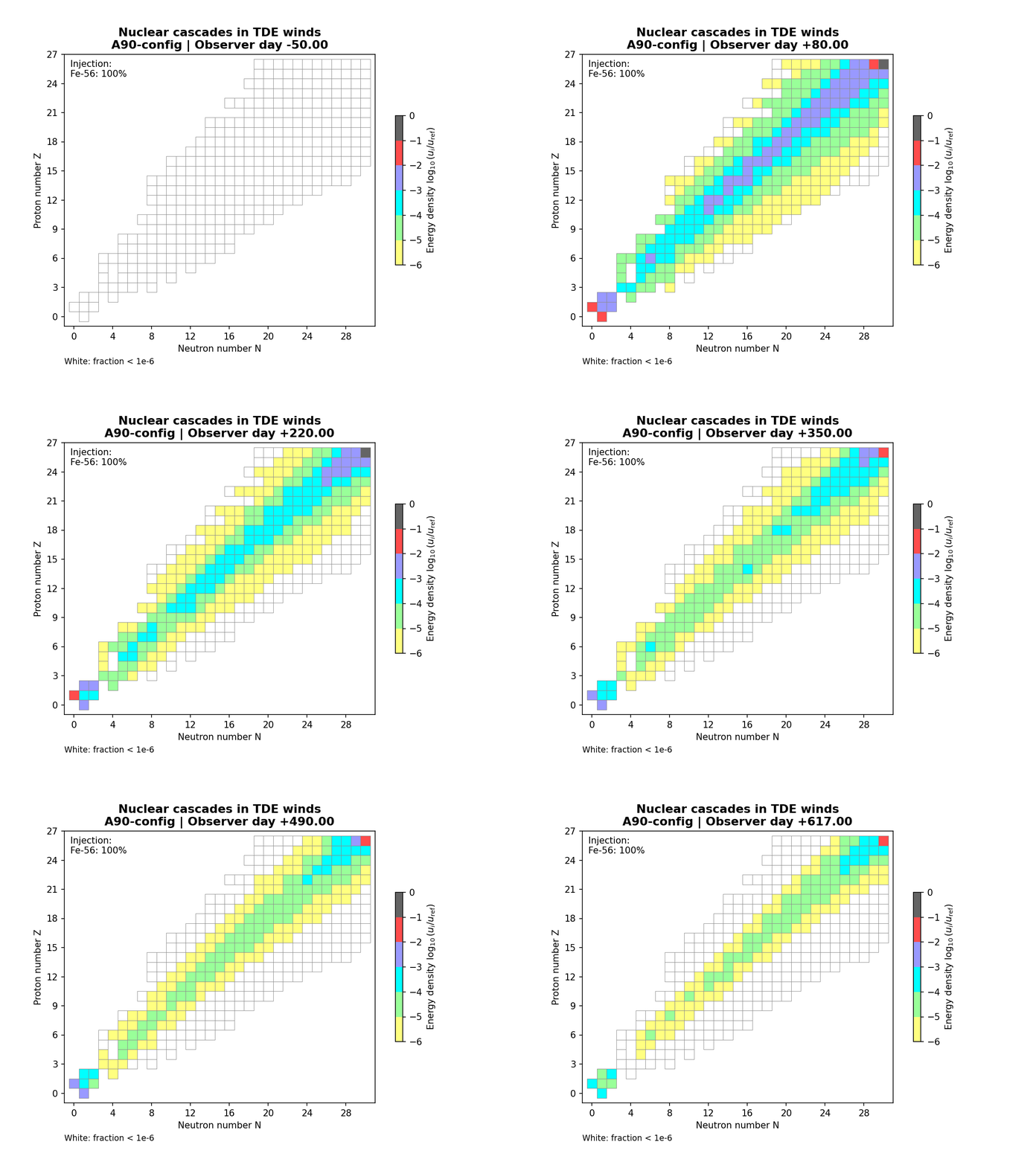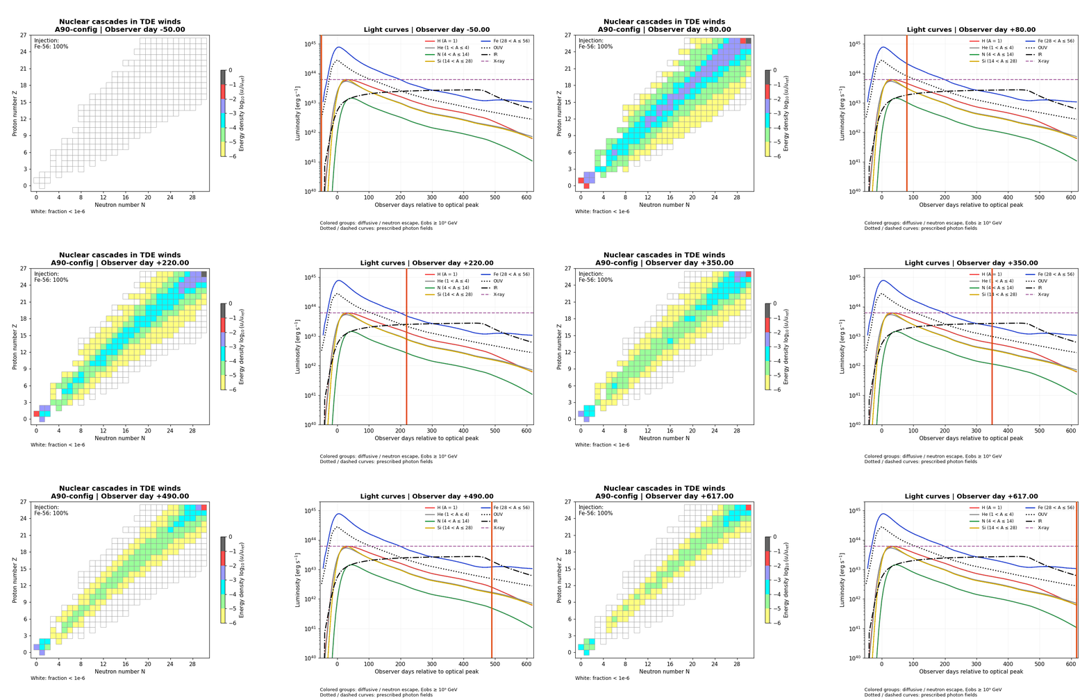
Time-dependent nuclear cascades with ANK

Chengchao Yuan, 2026/09/20

AstroNucleoKinetics (ANK) supplies nuclear interaction rates, secondary-production kernels, and single-species energy transport. NuCascade couples these calculations across a nuclear reaction network and evolves the differential number densities N_Z,A(E, t). Injected nuclei and their daughter nuclei can interact repeatedly, decay, lose energy, and escape. The same framework supports steady-state calculations and evolution with time-dependent injection and source conditions.

AT2019dsg: a transient radiation environment

In a tidal disruption event (TDE), stellar debris feeds an accreting black hole and can supply a luminous radiation field and an outflow. In the scenario illustrated here, energetic nuclei propagate through a magnetized interaction region associated with a TDE wind. Optical/UV radiation, infrared emission associated with the dust echo, and X-rays provide targets for nuclear interactions. The connection between these radiation fields, neutrinos, and escaping ultra-high-energy cosmic rays motivates the source models discussed by Plotko et al., Ultra-High-Energy Cosmic Rays from Neutrino-Emitting Tidal Disruption Events.

The figures show a local ANK/NuCascade calculation for AT2019dsg. The parameters below describe this example and its adopted source model, rather than quantities all independently determined by observations.

Physical conditions adopted in the illustrated calculation
Quantity	Model prescription
Geometry and magnetic field	Homogeneous spherical region with fixed radius R = 5 × 10¹⁶ cm, volume V = 4πR³/3, and magnetic field B = 0.1 G. This is the particle-interaction radius, not a fitted blackbody photospheric radius.
Time and redshift	Redshift z = 0.051. Evolution spans observer days −50 to +617 relative to the optical peak. Source-frame intervals obey Δt_src = Δt_obs/(1 + z).
Optical/UV target	Planck spectrum with fixed kT = 3.37 eV and a prescribed bolometric light curve, normalized to 2.8 × 10⁴⁴ erg s⁻¹ at the optical peak.
Infrared target	Planck spectrum with fixed kT = 0.1594 eV. Its luminosity follows the supplied infrared light curve, representing the delayed dust-echo component.
X-ray target	Planck spectrum with fixed kT = 72 eV and constant luminosity 6.2 × 10⁴³ erg s⁻¹ in this example.
Nuclear injection	Pure ⁵⁶Fe with Q_Fe(E, t) ∝ f(t)E⁻² exp(−E/E_cut). The cutoff rigidity is 3.5 × 10¹⁰ GV, giving E_cut ≈ 9.1 × 10²⁰ eV for iron. The peak injected power is 1.26 × 10⁴⁶ erg s⁻¹. The time-dependent injection normalization follows the supplied optical/UV accretion proxy.
Gas and wind	The target proton density varies with the same accretion proxy. The adopted prescription uses a 5 × 10⁶ solar-mass black hole, Ṁc² = 100L_Eddf(t), a wind mass fraction of 0.2, and wind speed 0.5c: n_p = 0.2Ṁ[R/(0.5c)]/(V m_p).

Each photon component is normalized through its bolometric energy density, u_γ(t) = L(t)/(4πR²c), so that ∫ εn_γ(ε, t) dε = u_γ(t). A luminosity at one photon energy is not used as the bolometric normalization. The three fixed spectral shapes are evaluated separately and combined with their time-dependent amplitudes. Optical/UV and IR luminosities are interpolated in log luminosity, while the injection proxy is interpolated in linear luminosity.

Physical processes in the cascade

Photodisintegration: interactions with the target photons remove nucleons or nuclear fragments from a parent nucleus. The resulting daughter nuclei enter the transport network and can undergo further reactions. This example uses the A90 photodisintegration and isotope/decay data and follows a reachable network of 343 nuclear species, rather than only the first generation of iron fragments.
Radioactive decay: unstable species feed their daughters through the selected decay network. Relativistic time dilation affects decay rates, allowing competition between decay, further interactions, and escape.
Photomeson production: sufficiently energetic particles interact with photons to produce pions and secondary nucleons. Nuclear photomeson production is treated with a SOPHIA proton/neutron superposition approximation, using nucleon interactions at the corresponding energy per nucleon. This replaces a dedicated nuclear photomeson table in this calculation.
Interactions with gas: collisions of energetic nuclei with target protons provide an additional pion source through the ANK proton–nucleus interaction model. Here the Sibyll-based treatment removes the incident nucleus catastrophically and supplies pion production, without following baryon regeneration from those collisions.
Continuous energy losses: Bethe–Heitler pair production and synchrotron radiation reduce particle energy and reshape the nuclear spectra. The example keeps the source radius fixed and includes no source adiabatic cooling. Bethe–Heitler energy losses do not by themselves constitute a calculation of the emitted pair radiation.
Escape: charged particles have an energy-dependent diffusive escape rate Γ_diff = min(c/R, c r_L/R²) and an advective rate Γ_adv = 0.5c/R. Neutrons escape at c/R. Both charged-particle escape terms act in the same evolution, while the corresponding escaping spectra are recorded separately.

What the time evolution resolves

The calculation begins with zero nuclear density and continuously injects iron as the source brightens and fades. NuCascade balances injection and secondary production against fragmentation, decay, cooling, and escape. Consequently, the nuclear population retains the history of earlier injection and interactions: its composition at a given time need not coincide with a steady-state solution for that instant. The evolving radiation field changes which interaction channels compete effectively with escape, while repeated reactions populate lighter nuclear species.

ANK supplies the microscopic rates and energy-transport solutions; NuCascade assembles the coupled network and advances it in physical time. Outputs include nuclear spectra, energy densities, composition maps, escaping-particle light curves, and integrated fluences. The animation below shows the species energy densities relative to a fixed reference normalization, preserving changes in the overall stored population as well as its composition.

Time evolution of the AT2019dsg nuclear cascade on the neutron-number versus proton-number plane — **Nuclear cascade evolution.** Each cell represents a nuclear species, colored by its energy density relative to the saved reference energy density. The animation follows the buildup and evolution of the nuclear population, including lighter fragments generated from iron. Observer time is measured relative to the optical peak; white cells lie below the displayed threshold.

Energy spectra and composition. Mass-grouped cosmic-ray spectra show time-integrated diffusive/neutron escape (left), advective escape (middle), and release of the population remaining at the end of the calculation (right). The ordinate is energy-weighted fluence, rather than instantaneous luminosity. Black curves show the total; dashed curves give the hypothetical free iron-56 reference.

Pion source terms and downstream radiation

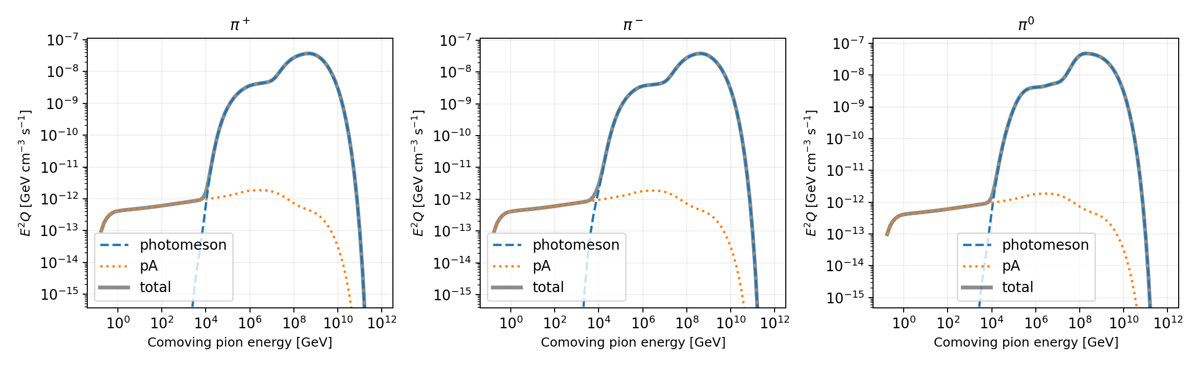
The calculation also exports the differential production rates Q_π⁺(E, t), Q_π⁻(E, t), and Q_π⁰(E, t) in cm⁻³ s⁻¹ GeV⁻¹, with separate photomeson and gas-collision contributions. These are injection source terms for a downstream radiation calculation, not cooled pion densities. An AM3 coupling can map the charged-pion sources onto its energy and time grids and convert neutral-pion decay into a photon source, then calculate pion/muon cooling and decay, electromagnetic cascades, and photon and neutrino emission. That coupling is not connected in the current DSG reproduction script, and the figures above show the nuclear-cascade calculation.

Scope of this example. The photon fields are prescribed, without radiation feedback from the cascade. Missing nuclear residuals use the configured nucleon-emission approximation. The displayed cosmic-ray fluences include source escape and cosmological redshift, but no intergalactic nuclear propagation. The final-release panel represents the population left at the end of the same evolution; it is distinct from the particles accumulated through continuous escape.

Open the animation · Open the spectra PDF